Protein three-dimensional structure is no longer solely the domain of specialists interested in the rules that govern the relationship between an amino acid sequence and its structure. The emphasis is changing from one in which such data are used to provide a structural framework for understanding biological function and mechanism to focusing on the application of such information for specific ends in areas such as molecular medicine, fine chemicals, agriculture and even biological electronics. The potential users of protein structures represent a growing population of non-specialists and it is of interest therefore that such information be brought to a wider audience.

It is not our intention here to provide an exhaustive treatment of all existing databases and programs applicable to questions of protein structure and their modelling. Indeed, with the current explosive growth of the field we are probably regretfully unaware of many useful facilities which may already exist. Our objective instead is to provide an introduction to the non-specialist and a brief guide to some of the most useful sites on the internet.

One of the problems facing a new user of any data is the degree of confidence with which one should treat it. Often one is interested in benefiting from the information provided without worrying about the intricacies of how it was obtained. Besides a description of some of the databases available, we therefore provide a brief guide to the errors and inaccuracies present in protein structures and how they can be conveniently evaluated. Subsequently we describe possible applications for such information in the form of molecular modelling.

There are basically only three experimental techniques capable of a complete structure determination of a biological macromolecule. These are (1) X-ray diffraction of single crystals (X-ray crystallography), (2) multidimensional NMR and (3) electron diffraction of two-dimensional crystals. The results are deposited in the form of formatted co-ordinate files in the Protein Data Bank (PD.) at the Brookhaven National Laboratory, USA[1]. In some cases, but not necessarily, the experimental data used to derive the structures is also made available. In 1995 the data bank contained approximately six times as many structures derived by crystallographic techniques than by NMR but the relative growth of the latter was greater. Table 1 shows some of the principal differences between the two techniques[2]. To date we are aware of only two complete structure determinations done by electron diffraction (bacteriorhodopsin[3] and the plant light harvesting complex[4]).

• Mathematically direct reconstruction of the image of the molecule (electron density map)
• Applicable to large proteins and complexes
• Data processing highly automated
• Well established quality indicators available (R-factor, resolution)
• Structured water can be determined
• Generally higher precision

• Applicable in solution (more biologically relevant)
• Better information about dynamics of the molecule
• Structures not influenced by crystal packing
• Can be applied to isolated domains or modules of larger proteins
• Physiological conditions can be readily altered (pH, temperature etc.)

Disadvantages:

• Need for stable well diffracting crystals
• Crystallisation techniques largely empirical
• Measurements made in the solid state (non-physiological)
• Need for ionising radiation which may cause radiation damage
• Difficulty in distinguishing static and dynamic disorder
• Loss of dynamic information and the tendency to `freeze' flexible regions within the crystal lattice

• In general the precision of the atomic co-ordinates is lower
• Limit to the size of the molecule that can be studied (<20kDa)
• Difficult to determine relative domain orientations in multidomain or modular proteins
• No single value analogous to the resolution of a crystal structure available to assess precision
• Requires concentrated solutions (non-physiological)

Table 1. Some of the relative merits and limitations of the two principal methods for the determination of protein three-dimensional structure (adapted from ref [2]).

A typical crystallographic co-ordinate file, identified by its PDB code (generally a number followed by three alphanumeric characters) consists of a header which includes the following type of information:

Following the header are the atom records which consist of 14 fields most of which are self-explanatory. After the atom serial number, atom name (CA for a -carbon etc.), 3-letter amino acid code, chain identifier and residue number come the Cartesian co-ordinates (x,y,z) followed by the atomic occupancy and B-factor (temperature factor). Despite the co-ordinates being quoted to a precision of a thousandth of an Å ngstom unit, this is greatly in excess of the real precision of the structure. The occupancy will normally be 1.000. If it is not, this may mean that a particular atom can have one of several positions in the crystal (due for example to a disordered side-chain) in which case there will be more than one record for the same atom. If the occupancy is zero, it means that the atom has been `modelled' (see below) probably using stereochemical criteria alone and not included in the refinement. Such regions should be treated with great caution! The B-factor represents the degree to which a particular atom is statically or dynamically disordered. The higher the B-factor, the greater the disorder and this corresponds to a greater probable error in the co-ordinates. The well-determined parts of the structure will typically have B-factors below 20Å 2. Where B reaches values above 50Å 2 the structure should be treated with greater caution. It may indicate other possible conformations for the structure which are not presented.

Atoms which are not part of normal amino acids are identified by HETATM records. They may be metal ions, water molecules, inhibitors etc.

Co-ordinate files for structures determined by NMR are essentially identical to crystallographic files but with some modifications. Often co-ordinate sets corresponding to several different (typically 20) structures are deposited (a so-called ensemble). These correspond to the structures most compatible with the experimental NMR restraints. Sometimes a single best or average structure is deposited. Several of the above-mentioned parameters such as resolution and R-factor are not applicable to NMR structures. There is in general a correspondence between highly variable regions in an NMR ensemble and regions which present high temperature factors in crystallographic studies, though it is clear that the crystal lattice restrains the movement of such regions more than in solution.

A small percentage of PDB files represent modelled structures. We should make a very clear distinction between such structures and those described above which have been experimentally determined by X-ray crystallography, NMR or electron diffraction. Modelled structures are hypothetical in nature and not directly based on experimental data. Such models are normally produced by homology modelling (see below) using knowledge-based techniques, by comparison with known structures of other members of a given protein family. Such models may represent reasonably well the structure in the conserved core but in general should be treated with considerable caution.

On the 12th August 1996 the PDB contained 4707 entries, 4368 of which were protein structures, 327 nucleic acids and 12 carbohydrates. The data bank currently doubles in size roughly every 2 years and there are predictions that by the end of the decade the rate of structure determination will reach 2 structure per hour [5]. It can be accessed by WWW at http://www.pdb.bnl.gov. The PDB-Browser allows for searching over PDB records using search strings and Boolean functions. The results of searches can be downloaded to the user's home computer and visualised. Programs such as RasMol[6] and Mage for molecular visualisation and manipulation of structures are available for PC, Macintosh and Unix workstations. (RasMol can be obtained by anonymous ftp from ftp.dcs.ed.ac.uk in the directory /pub/rasmol or from the PDB at ftp.pdb.bnl.gov in /pub/other-software/Rasmol and Kinemage from ftp.pdb.bnl.gov in /pub/kinemage). On the PC and Macintosh RASMOL manipulates molecules faster than MAGE and can also handle NMR ensembles.

Furthermore, annotated images of structures in the PDB can be visualised and downloaded from the following sites: http:/expasy.hcuge.ch/pub/Graphics/ or ftp://pdb.pdb.bnl.gov/images/GIF and ftp://pdb.pdb.bnl.gov/images/RGB or via the PDB-Browser. The images have been produced using the program RIBBONS[7] and are aimed at being illustrative, allowing ready familiarisation with a given protein of interest. Several views are provided, at least one of which is in stereo.

Alternative and convenient access to the information present in the PDB are the so-called Molecular Modelling Database (MMDB) on the Entrez server at NCBI and Moose at the San Diego Supercomputer Centre. MMDB is a compilation of all the PDB 3-dimensional structures of biomolecules as ASN.1-formatted records, not PDB formatted records. MMDB-Entrez can be accessed at http://www3.ncbi.nlm.nih.gov/htbin-post/Entrez/ and Moose at http://db2.sdsc.edu/moose/ .

Mirror sites of the PDB exist in Europe at the European Bioinformatics Institute -EMBL outstation in Cambridge, at the Institute of Physical Chemistry, Beijing, China and at the Weizmann Institute of Science, Israel. The appropriate URL's are given in the appendix. In our experience access from South America is normally easiest to the USA.

Many of the entries in the PDB are for the same protein. They may differ in the crystal form used (which itself may represent differences of pH, precipitant concentration etc.), the refinement protocol used, the presence of inhibitors or cofactors etc. Furthermore there are many examples of structures for different proteins from the same family. For some applications this wealth of information is extremely important for understanding macromolecular action but for others a reduced non-redundant database would be of interest. Several attempts have been made to reduce the PDB to a representative set of a few hundred structures[8,9]. Such lists are available by anonymous ftp from ftp.embl-heidelberg.de in the directory /pub/databases/protein_extras/pdb-selectm of from the web page http://www.sander.embl-heidelberg.de/pdbsel/ .

Experimentally determined crystal and NMR structures are subject to the same types of error which can affect any experimental measurement. In the case of protein crystallography these can be both random and systematic errors affecting the measured intensities of the diffracted X-ray beams. Furthermore not all of the information necessary for reproduction of the molecular structure can be directly measured. The missing part (the phases of the diffracted beams) has to be recovered indirectly and there are normally large errors associated with their estimation. To complicate matters further, at the stage of interpretation of the electron density map considerable human intervention is necessary. All of these factors can lead to errors in the final structure which can be small random co-ordinate errors, incorrect side-chain rotamers, peptide bond flips, regions where the structure becomes out of register with the structure, reversed directionality of elements of secondary structure and incorrect connectivity of such elements leading to an erroneous topology [10]. Such errors are normally a function of resolution.

Besides the traditional quality indices described above (R-factor, stereochemistry etc.) for crystal structures, several other useful checks can be performed on PDB files in order to get an overall appreciation of the quality of the structure.

Amongst the quality control programs currently available are PROSA[11], PROCHECK[12], VERIFY_3D[13], QUALTY[14] (WHATIF[15]), Holm & Sander[16] etc. PROCHECK performs a complete set of stereochemical evaluations including bond angles and lengths, peptide bond planarity, Ca tetrahedrality, H-bond energies, side-chain rotamers and Ramachandran plots. The latter is sometimes sufficient in itself to distinguish between a well determined structure and one which presents stereochemical problems (see Fig. 1). Ideally a well-determined structure will have > 90% of its residues in the most favoured (darkest) regions of the Ramachandran plot. A PROCHECK analysis of a structure can be performed by submitting to the following web site:

PROSA calculates an energy graph of the structure as a function of amino acid sequence position. Peaks in the energy profile are indicative of problematic parts of the structure which should be treated with caution. The program is available from

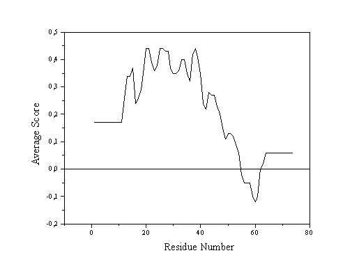
The quality control option of the graphics program WHATIF and the VERIFY_3D program from the laboratory of David Eisenberg evaluate the quality of three-dimensional structures with reference to the adequacy of the chemical environment around each amino acid residue. In the case of WHATIF the comparison is made between the atomic distribution around each rigid sub-fragment of each residue and that encountered in a standard distribution calculated from well-determined structures. VERIFY_3D adopts a similar but simplified approach in which negative values imply badly folded or otherwise problematic regions of the structure (Fig. 1). WHATIF incorporates other checks into a more complete package.

A useful facility for checking of protein structures is to be found at the Protein Structure Verification-Biotech Server at the following URL's http://biotech.embl-heidelberg.de:8400 or http://biotech.pdb.bnl.gov:8400. This is the result of an EC funded collaboration and will perform the PROCHECK and WHATIF checks as well as an atomic volume calculation (SurVol program).

Figure 1 - On the left are shown VERIFY_3D profiles and on the right Ramachandran plots (calculated using the program PROCHECK) for two protein structures deposited in the PDB. Above are shown results for the coordinate file 1MSA (snowdrop lectin) and below 2ABX (neurotoxin). The former presents an all-positive VERIFY_3D proifile and good steroechemictry (the majority of the backbone torsion angles f and y are within the most favoured (darkest) regions). The latter on the other hand shows a negative region towards the C-terminus of the VERIFY_3D plot and several stereochemical problemas as evidenced by the almost random distribution of points on the Ramachandran plot.

It is convenient to describe protein structure with reference to a hierarchy which at its most elementary level consists of the amino acid sequence (primary structure) and leads, at its most elevated level of organisation to the arrangement of subunits within oligomeric proteins (quarternary structure). Between these two levels, the secondary structure describes repetitive regions of the polypeptide backbone and the tertiary structure describes the three-dimensional fold. Several methods are available for the automatic definition of secondary structure from a PDB style co-ordinate file. Probably the most widely used is that due to Kabsch and Sander [17] which defines secondary structure solely on the basis of an energy criterion for hydrogen bonds. Their program (DSSP) and accompanying database can be accessed at http://www.sander.embl-heidelberg.de/dssp/ . A useful modification to DSSP is the program SECSTR which produces a definition which is more in line with that intuitively produced by crystallographers and NMR spectroscopists. SECSTR is part of the PROMOTIF [19] package available by anonymous ftp from 128.40.46.11. Information can be found at the URL:

Information on preferred tertiary structure interactions, in the form of the 400 possible residue-residue interactions can be found in the database of Singh and Thornton[18] at the following URL:

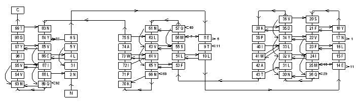
PROMOTIF [19] provides a means to analyse a wide variety of structural features in any given protein. Besides regular secondary structures (which may be plotted as schematic H-bonding diagrams, fig 2 [20]) PROMOTIF identifies disulphide bridge conformations, b and g -turns, bulges etc. and can be used to directly compare structures in order to identify structural differences.

The rapid growth in the rate at which protein structures are determined has led to a need for their more rational classification. Several attempts have been made in this direction and the relevant web sites can be found in the appendix. CATH[21] is an example of one such attempt and in common with most methods is based on the original efforts of Levitt and Chothia [22] and uses both automated algorithms and visual inspection.

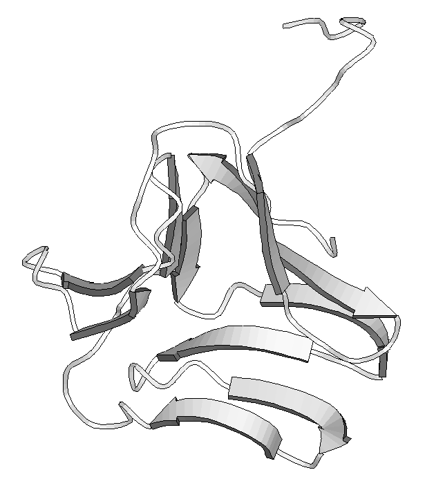
Figure 2. - Different ways to represent protein structures. On the left are shown HERA diagrams and on the right a MOLSCRIPT representation for two proteins from the Protein Data Bank (PDB). Above triose-3-phosphate isomerase and below, snowdrop lectin. The former demonstrates the typical TIM barrel fold found in several proteins of the glycolitic pathway . The latter shows a particular type of b -prism fold showing a local 3-fold pseudo-symmetry.

CATH is an acronym derived from the hierarchy used for the classification (Class, Architecture, Topology, Homology-see table 2). CATH can be accessed at the web site http://www.biochem.ucl.ac.uk/bsm/cath/CATHintro.html

and provides a useful research tool for the study of relationships amongst protein structures. If a given structure is of particular interest to a researcher, CATH represents a convenient means to rapidly identify related structures which often have related functions. Such knowledge may be of relevance to the subsequent development of the project.

• The highest level of the classification, derived from gross secondary structure content (a , b , a /b etc.).

• Description of the gross arrangement of secondary structures.

• Topological description, with reference to previously observed structures and well-known folds.

• Discrimination between structures with same topology, but more diverse structures.
• Often correlates with functional homology.

Finally there is a level grouping structures whose members show high percentage sequence identities

Sequence Family

• Greater than 30% sequence identity.
• High probability of having similar structure/function.

Table 2. The CATH classification of protein folds.

SCOP (Structural Classification of Proteins) is a similar system developed at the University of Cambridge but is less automated in nature and gives more weight to established evolutionary and functional relationships[23]. An example of the hierarchical nature of its organisation is illustrated in Fig. 3. The d -endotoxin superfamily presents a b -prism I fold in which three 4-stranded sheets lie approximately parallel to a pseudo-3-fold axis. They are therefore members of the all-b class. For more complex examples deeper levels (family and domain) exist within the tree structure. SCOP can be accessed at

The FSSP [24] classification of the Sander group at EMBL is totally automated and uses both sequence and structural alignments. A dendrogram describing the relationships is accessible at http://www.embl-heidelberg.de/dali/fssp .

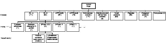
Figure 3. An example of a SCOP hierarchy.

its constituent domains remains a considerable problem as it is difficult to decide upon an unambiguous definition of what constitutes a domain, they having traditionally been defined by visual inspection of the structure. A recent and useful contribution has been made by Islam et al. [25] and their definitions applied to a non-redundant dataset are available by anonymous ftp from ftp.icnet.uk in the directory icrf-public/bmm/domains.

On determining a new structure it is often of interest to know if a similar fold has been observed previously. This may not represent a problem if the protein is a member of a well-known family or presents a classic topology (a (b /a )8 TIM barrel or a four-helix bundle for example). However, in many cases it is not obvious if a fold has been seen previously or which are the most related structures. Programs to perform such three-dimensional comparisons are obviously of great value in simplifying such a task. Many such methodologies have been described[26] and ideally they should be able to identify similar substructures in proteins of very different overall size and be rapid enough to search large databases. The Dali (Distance Matrix Alignment Program) server is one such example. PDB format files may be submitted to dali@embl-heidelberg.de which will be compared with the representative subset of the Brookhaven Data Bank. Full instructions can be found at http://www.embl-heidelberg.de/dali/dali.html . Other methods such as that of Taylor which uses the dynamic programming approach used to derive CATH[27] and the PROTEP[28] program of Artymuik which employs graph theory are also of interest.

Several data storage and retrieval systems for protein structure have been described. They are more or less complex in nature and differ in the way in which the data is pre-processes and organised in order to speed up retrieval[29-31]. An ideal system for researchers interested in what governs protein three-dimensional structure or in the detection of uncommon features of a given structure for example, is one which permits the formulation of complex questions of the type `what is the frequency of occurrence of buried cysteines involved in disulphide bridges linking two a -helices?' The database Iditis commercialised by Oxford Molecular and available for example on the Daresbury laboratory SEQNET computer, permits such queries. A similar system (SCAN3D) is part of the WHATIF program mentioned previously.

One of the most exciting developments in the field of protein structure and its prediction over the last few years has been the observation that sequences which apparently present no obvious homology, often present remarkably similar folds. This has led to a plethora of methods for fold identification directly from amino acid sequences. In general the approach involves the comparison of the sequence of interest against a data bank of representative folds[32]. It is thus quite distinct from the methods described above for structure-structure comparison.

Such methods for `threading' (or 1D-3D comparison) are variable in their form. Probably the most successful as judged by the recent protein structure prediction meeting held in Asilomar in 1994 are those of the groups of Thornton in London[33] and Sippl in Salzberg[34]. The former program (THREADER) can be obtained from

and a graphical user interface for assessment of the results can be obtained by ftp from ftp.biochem.ucl.ac.uk in the directory pub/px. (In this context it is well worth consulting the University College biomolecular structure group's homepage whose URL is http://www.biochem.ucl.ac.uk/bsm/index.html ). Enquiries concerning the Salzberg method should be sent to Manfred Sippl at the Centre for Applied Molecular Engineering (sippl@agnes.came.sbg.ac.at).

These techniques offer the possibility to identify structures for new sequences which are not homologues of any member of the PDB. In the case of sequences resulting from genome projects for which no function may be known, the identification of a fold may represent the first indication of a possible biological role. Other methods available on the WWW include that of SARF at http://www-lmmb.ncifcrf.gov/~nicka/sarf2.html .

Clearly protein (or more generally biological macromolecular) databases are not the only molecular structure databases available. Basically four crystallographic databases cover the spectrum from metals and alloys, inorganics and minerals, small organic and metallo-organic structures (the Cambridge Structural database, CSD)[35] and proteins (PDB). The CSD holds details of over 150,000 principally small molecule structures (April 1996). Such databases and the information contained therein are becoming increasingly important for structural molecular biologists interested in the use of protein structure for example in drug design. In such circumstances the investigator will generally be interested in the interaction between a small molecule (a potential inhibitor or drug) and a protein receptor and will require structural information about both.

The CSD includes one-dimensional information in the form of compound names, molecular formulas, bibliographic references etc., two-dimensional information such as chemical connectivities and structural diagrams and three-dimensional information in the form of atomic co-ordinates and crystallographic parameters. Additionally all non-co-ordinate information from the PDB has recently been included and a new database (CSDUse) contains references to CSD applications. An interactive graphics package provides an interface to the database and is composed of three programs QUEST3D, VISTA and PLUTO. The former is the mains search program permitting the retrieval of 2D substructures which may be further constrained by geometrical criteria and the location of non-covalent intermolecular contacts amongst many others. The searches can be made graphically and the results (torsion angle distributions which describe conformational preferences for example) analysed by the program VISTA.

Much information on the CSD, its related programs and many other similar systems or complementary software can be obtained from the homepage for the recent Erice meeting on structure based drug design (http://www.organic.emory.edu/ccsem/ ). The URL for the Cambridge Crystallographic Data Centre can be found in the appendix.

We mentioned in section 2.3 that a small fraction of PDB files represent `modelled' and not experimentally determined structures. Such models are normally derived by `homology modelling'. The fundamental justification for such techniques is the observation that proteins 3D structures are better conserved amongst members of a homologous family than are their amino acid sequences[36]. This general statement leads naturally to the conclusion that if homology can be detected between two sequences at the level of the amino acid sequence then the three-dimensional structure of the two proteins should be similar. If one of the structures is known experimentally then a model for the second can be derived using knowledge-based techniques[37].

Figure 4 demonstrates schematically the stages involved in the construction of a homology model. Initially all homologous structures to the sequence being modelled are retrieved by standard data bank searching techniques. A `structure-based' alignment is derived from such structures usually by rigid-body superposition although more sophisticated methods exist which cope better with multidomain proteins where the relative orientation of domains may vary from one member of the family to another [38]. The sequence of interest may subsequently be included in the alignment by applying restraints which force the insertions and deletions (indels) to the loop regions outside the elements of secondary structure (alignment programs such as MULTALIGN[39] readily allow for such restraints). Alternatively the `common core' of the family can be determined automatically from the structural superposition using, for example, a maximum deviation criterion[40].

Figure 4. Schematic representation of the stages envolved in the modelling of a protein structure by knowledge-based techniques (homology modelling). Starting from a final alignment including known 3D structures and the sequence of interest, the common core, loops and side-chains are constructed leading to a model which may be minimized and evaluated. The results of such sterochemical, packing and atomic contact analyses can be used to guide further cycles of the modelling process until the procedure converges on a final structure.

Residues might be considered part of the common core if their Ca positions lie within a given distance (say 3Å ) of one another. Indels are then maintained outside of the common core as it is expected that this region will be similarly conserved in sequence being modelled.

The construction of this common core can take three basic forms. In one approach, a single structure from amongst those known experimentally may be taken as the basis structure for the model. In such cases the choice will probably be governed by the percentage sequence identity with the sequence being modelled or the resolution/R-factor of the structure. Alternatively, a weighted mean of the core regions from all known structures may be taken, weights once again being assigned to the individual structures on the basis of their sequence identity for example[41]. A third possibility would be to use a `spare parts surgery' approach, in which different parts of the core are taken from different structures. If only one 3D structure is available then there is no choice in the method to be adopted.

The production of the core provides the framework for the modelling of the variable regions which normally correspond to the loop regions between secondary structure elements. Several techniques exist for such applications. They vary from loop searching in a database of well refined structures using geometrical restraints derived from the core regions[42] to the use of ab initio and molecular dynamics techniques[43]. Several criteria must be applied to the acceptance of a given possible loop conformation. Such criteria include for example the adequacy of the interactions made between the loop and its neighbouring structures and the backbone conformation for the sequence of residues in the loop itself.

Once established the complete backbone conformation the side-chains may be included in the model. Normally the rotamers for the side-chains are chosen on the basis of identical or chemically similar residues in the equivalent position in homologous structures or with reference to secondary structure dependent preferences[44,45] or more sophisticated searching techniques which depend on the local backbone conformation[46].

In order to remove steric impedance in the completed model, the structure is subject to a debumping procedure using a torsional driver and/or energy minimisation employing standard force fields. The final model may be evaluated using the same techniques as described in section 3.2.

During the recent Asilomer meeting [47] several homology built models were evaluated by comparison with their previously unpublished crystal structures. Several of the models were built by completely automated procedures. The program MODELLER appears to be one of the most successful although it adopts a somewhat different approach to that described above[48]. It is available by anonymous ftp from

Swiss-Model is an automated homology modelling program available by email which uses the ProMod program[49]. When supplied with a sequence it will initially determine if homology modelling is possible (first approach mode) and if so produces a first attempt model and requests the files necessary for model optimisation. The optimise mode will fine tune the original attempt using additional input from the user (the tweaking of sequence alignments etc.) The approach adopted is similar to that described above for interactive modelling. After identification of the available homologous structures, the common core is built by the averaging procedure described above and database searches used for loop construction and side-chain building. The model is energy minimised using CHARMM[50] and evaluated using similar techniques to those described in section 3.2.

The facility is available from the ExPASy molecular biology server

and promises a turnaround of about an hour. However, currently only an approximately 25% of sequences are amenable to homology modelling and of these less than half can be considered reasonably reliable[51].

A final word of warning is that all such models should be treated with great caution as they are hypothetical in nature. Automated procedures (like those that depend on manual intervention and intuition) will fail in many situations as the problems to be overcome are complex and interdependent and challenge our current understanding of the factors that determine the native folds of proteins. However, even `low resolution' models which present co-ordinate errors may still be of value in some circumstances for planning subsequent experiments and testing hypotheses. Often such a model is considerably better than nothing.

HSSP[52] (http://www.sander.embl-heidelberg.de/hssp/) was probably one of the first implicit databases of models. In fact it is a database of alignments of homologous sequences to known structures. The `models' are implicit in that they are described by amino acid equivalences in the form of the alignments and not `explicit' in the form of 3D atomic co-ordinates. 3D_ali [53] uses a similar concept but matches sequences to multiple structures rather than to individual PDB entries. As a consequence it is somewhat less redundant. It can be accessed at http://www.embl-heidelberg.de/argos/ali/ali.html .

A database of automatically generated models using the ProMod program described above is available at the ExPASy server (http://expasy.hcuge.ch/cgi-bin/swmodel-search-de) allowing the user to perform searches in order to identify pre-constructed models for sequences of interest. It is worthwhile checking this database prior to embarking on the construction of a model since one may already exist and be sufficient for ones purposes.

It is clear that with the rate of structure determination world-wide reaching one co-ordinate set every 30 minutes by the end of the decade, the era in which the determination of a protein structure was considered a considerable experimental obstacle has passed. If such a prediction is realistic and if all crystallographic and spectroscopic effort were solely devoted to a single genome project for example, it would in principle be possible to determine the structures of all the expected proteins of the human genome in approximately five years. This does not mean that all structure determinations have become trivial. In particular the bottleneck of protein crystallisation for X-ray diffraction experiments is expected to be a continuing problem. However, it does mean that there is a new emphasis being placed on what to do with the vast amount of structural information being provided by structural molecular biologists. Clearly the adequate organisation of such information and its efficient access are fundamental to its best utilisation. It is therefore expected that the area of bioinformatics will continue to grow in the coming decade and that protein and small molecule structures together will find ever increasing applications in fields such as the design of new pharmaceuticals, biotechnology and bioelectronics.

[1] Bernstein, F.C. et al. (1977) J. Mol. Biol. 112, 535-542

[2] MacArthur, M.W., Driscoll, P.C. & Thornton, J.M. (1994) Trends. Biotech. 12, 149-153

[3] Henderson, R. et al. (1990) J. Mol. Biol. 213, 899-929

[4] Kuhlbrandt, W., Wang, D. & Fujiyoshi, Y. (1994) Nature 367, 614-621

[5] Wodak, S.J. (1996) Nature Str. Biol. 3, 575-578

[6] Sayle, R.A., and Milner-White, E.J. (1995) TIBS 20:374-376.

[7] Carson, M. & Bugg, C.E. (1986) J. Mol. Graph 4, 121-122

[8] Boberg, J.,m Salakoski, T. & Vihinen, M. (1992) Proteins: Structure, Function and Genetics 14, 265-276

[9] Hobohm, U & Sander, C. (1994) Prot. Sci. 3, 522-524

[10] Brändén, C-I. & Jones, T.A. (1990) Nature 343, 687-689

[11] Sippl, M. (1993) Proteins: Structure, Function and Genetics 17, 355-362

[12] Laskowski, R.A., MacArthur, M.W. & Thornton, J.M. (1993) J. Appl. Cryst. 26, 283-291

[13] Lüthy, R., Bowie, J.U. & Eisenberg, D. Nature 356, 83-85

[14] Vriend, G. & Sander, C. (1993) J. Appl. Cryst. 26, 47-60

[15] Vriend, G. (1990) J. Mol. Graph. 8, 52-56

[16] Holm, L. & Sander, C. (1992) J. Mol. Biol. 225, 93-105

[17] Kabsch, W. & Sander, C. (1983) Biopolymers 22, 2577-2637

[18] Singh, J. & Thornton, J.m. (1992) Atlas of Protein Sidechain Interactions Vol I & II, IRL Press, Oxford

[19] Hutchinson, E.G. & Thornton, J.M. (1996) Prot. Sci. 5, 212-220

[20] Hutchinson, G.E. & Thornton, J.M. (1990) Proteins: Structure, Function & Genetics 8, 203-212

[21] Orengo, C.A., Flores, T.P., Taylor, R.W. & Thornton, J.M. (1993) Prot. Eng. 6, 485-500

[22] Levitt, M. & Chothia, C. (1976) Nature 261, 552-558

[23] Murzin AG, Brenner SE, Hubbard T, Chothia C. (1995). J. Mol. Biol. 247:536-540.

[24] Holm, L & Sander, C. (1994) Nucl. Ac. Res. 22, 3600-3609

[25] Islam, S.A., Luo, J. & Sternberg, M.J.E. (1995) Prot. Eng. 8, 513-525

[26] Orengo, C. (1994) Curr. Op. in Struct. Biol. 4, 29-40

[27] Taylor, W.R & Orengo, C.A. (1989) J. Mol. Biol. 208, 1-22

[28] Grindley, H.M., Artymiuk, P.J., Rice, D.W. & Willett, P. (1993) J. Mol. Biol. 229, 707-721

[29] Bryant, S.H., (1989) Proteins, 5, 233-247

[30] Vriend, G. (1990) Prot. Eng. 4, 221-223

[31] Islam, S. & Sternberg, M.J.E. (1989) Prot. Eng. 2, 431-442

[32] Lemer, C. M-R., Rooman, M.J. & Wodak, S.J. (1995) Proteins 23, 337-355

[33] Jones, D.T., Taylor, W.R. & Thornton, J.M. (1992) Nature 358,86-89

[34] Flöcker, H., Braxenthaler, M., Lackner, P. Jaritz, M., Ortner, M. & Sippl, M.J. (1995) Proteins:

Structure, Function & Genetics 23, 376-386

[35] Allen, F.H. et al.(1991) J. Chem. Inf. Comput. Sci. 31, 187-204

[36] Bajaj, M. & Blundell, T.L. (1984) Ann. Rev. Biophys. Bioeng. 13, 453-492

[37] Blundell, T.L., Sibanda, B.L., Sternberg, M.J.E. & Thornton, J.M. (1987) Nature, 326, 347-352

[38] Sali, A. & Blundell, T.L. (1990) J. Mol. Biol. 212, 403-428

[39] Barton, G. (1990) Meth. Enz. 183, 403-428

[40] Blundell, T.L. et al. (1988) Eur. J. Biochem. 172, 513-520

[41] Srinivasan, N. & Blundell, T.L. (1993) Prot. Eng. 6, 501-512

[42] Jones, T.A. & Thirup, S. (1986) EMBO J. 5, 819-822

[43] Moult, J. & James, M.N.G. (1986) Proteins, Structure, Function & Genetics 1, 146-163

[44] McGregor, M.J., Islam, S.A. & Sternberg, M.J.E. (1987) 198, 295-310

[45] Dunbrack, Jr., R.L. & Karplus, M. (1993) 230, 543-574

[46] Vriend, G., Sander, C. & Stouten, P.F.W. (1994) Prot. Eng. 7, 23-29

[47] Mosimann, S., Meleshko, R. & James, M.N.G. (1995) Proteins: Structure, Function & Genetics 23, 301-

317

[48] Sali, A. & Blundell, T.L. (1993) J. Mol. Biol. 234, 779-815

[49] Peitsch, M.C. et al. (1993) Int. Immunol. 5, 233-238

[50] Brooks, B.R. et al. (1983) J. Comp. Chem. 4, 187-217

[51] Peitsch, M.C. (1995) Biotech. 13, 658-660

[52] Sander, C. & Schneider, R. (1991) Proteins 9, 56-68

[53] Pascarella, S., Milpetz, F. & Argos, P. (1996) Prot. Eng. 9, 249-251

CATH - structure neighbors, fold classification and

3D-viewing

SARF - structure neighbors, fold classification,

similarity search service

SCOP - structure neighbors. fold classification and

3D-viewing

ExPASy - Molecular Biology server

The DSSP program and database

The HSSP database

3D_ali

SWISSPROT protein sequence database

GDB - Genome Data Base

GenBank-NIH Genetic Sequence Database

O Home Page

PDB - Protein Data Bank

Non-redundant PDB

PDB Mirrors: EBI, Cambridge

IPC, Beijing

Weizmann Inst, Rehovot

Pedro's BioMolecular Research Tools

PIR-Protein ldentification Resource

Protein Structure Verification-Biotech Server

Promotif

Dali

MOOSE - Macromolecular Structure Database

MMDB-Entrez